You fulfilled your promise and published this video. Thanks a lot Mike. I have tried to achieve this task yesterday and I got it done but it took me some time. I was delighted that it worked out.
Glad to hear that you figured it out on your own! That means you are quite Excel Smart : ) Thanks for your support of this excelisfun channel at UA-cam : )
Well, thanks to my best teacher Mike who is more than amazing. The most important thing I learned from you is mastering the logical tests in Excel. I was a blind user of Excel before discovering your channel... Thanks. 👍 🌟 🌟
Wow, the fact that you added a homework for us to practice is so great, that's just what I needed! I was planning to do some revision test after the third episode myself and you just made it a lot easier! Thank you so so much for your videos, they made Excel really fun to me. I'll have so many new opportunities in my work life thanks to you! Just once again, thank you very much :)
Just me making videos, but you do not need words to express your gratitude, all I ask is for you to shown your support with a comment and thumbs up on each video that you watch, and a Sub too. Thanks, CA.Lakshmi Narayan Reddy Jambula !!!!!
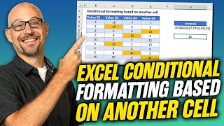
Thanks, Chris! This is one of the first times I have did not use cells to show logical formula, first, then put the formulas in the Conditional Formatting Dialog box. Using cells to show logical formula IS a more effective teaching method because we can visualize the patterns of TRUEs and FALSEs, but I am trying these shorter videos and acutally, many viewers do not want the why, just the how, and this video cust to the chase and shows quickly the how.
Very nice trick, and very helpful! You see I'm totally right when I said that excelisfun is the right place to learn excel, and not just that but how to have the fun with it 🙂👍
Good vid, Mike. When composing formulas in that edit box, I often go to move the cursor with the keyboard and it goes all psycho. I've learned to press F2 before trying to navigate in the edit box.
@@excelisfun Hi Mike.. thanks.. yes.. it is a great way to help the user visualize selections, as you have shown in your example. A variation I use is when interrogating a large and or long list where it is easy to lose track of the row, column and cell you are on. I set up CF as follows: Rule 1: =CELL("address")=ADDRESS(ROW(),COLUMN()) Rule 2: =CELL("col")=COLUMN() Rule 3: =CELL("row")=ROW() Then I write a small macro into the worksheet_SelectionChange event as follows below. I name my target range myRange and use the If Not Intersect is Nothing method to keep the code from running when the pointer is outside the table (credit to Leila G. for teaching me this): Private Sub Worksheet_SelectionChange(ByVal Target As Range) If Not Intersect(Target, Range("myRange")) Is Nothing Then ActiveSheet.Calculate End If End Sub So, this produces a moving crosshair wherever the cell pointer is positioned and makes it easy to keep track of where I am in the list. The only downside is a performance lag on large tables. But, it can be a big help if you have many columns and rows. It's too bad MS does not make this a feature option to turn on/off from the ribbon menu without having to use CF and write a macro. I think it could be a useful feature built right into EXCEL.. the crazy crosshair or crosshare.. haha!!
Mike, yes. And it works as advertised. If a particular cell has been formatted by a rule, no need to evaluate the other rules for that cell. In several types of templates I use quite a lot of mutually exclusive rules (IF this letter THEN that background color): no need to evaluate all the rules: as soon as it finds the one TRUE rule, it can stop. In your case here, because of the overlapping rules: the order matters (anyway).
Can this be modified to use the currently active cell position? I'd try myself, but at the moment I do not have access to any MS Office. I have seen the use of a VBA macro and using the selection change event and .Select to select the row & column of the cell that is currently selected, but that messes up the user experience big time. Thank you!
Help me for this I want conditional formatting for Row and Column upto at intersection cell, and beyond intersection cell no highlighting like Mirror L not like +
Similar to my problem: Month names in row 1, day numbers down column a, year in cell A1, I want conditional formatting of weekends, updated as year changes.
I have more than 10k rows filled with data and I want to search specific value location (row/column number) based on input I enter, input will be two different value. could you please help how to do this
hi Mike ... my office 365 has updated recently .... and i found while checking its options that there is a new com addins called "Data Streamer" .... What is it ?!!!
I have no idea!?!?! I just Googled it and it said: Data-Streamer. Data-Streamer is a two-way data transfer Excel add-in that streams live data from a microcontroller into Microsoft Excel and sends data from Excel back to the microcontroller. It opens the emerging world of IoT to the classroom and helps educators meet the NGSS and ISTE requirements for data science. support.office.com/en-us/article/data-streamer-c90aebcf-3d44-47ab-a068-549a0b9edfc6 But I still did not understand it when I went to the Microsoft Help Link (typical).
I am sorry, jai, but i will not do that. The first 1000 videos that I made (most of whcih are not at UA-cam) were with face cam, but then I developed editing and teaching techniques that emphasize the action of creating the formulas more than what is going on with my face. So I do not use face cam. Sorry about that : (
ExcelIsFun :-A question for You .A Bank stock price is moving from 100 to 300 in Last five Years. I want to Find Dates when ever it Touches price 180 With vlookup.I have Dates in column A & closing price in column B...
Phone Excel, I got this message by e-mail: ExcelIsFun :-A question for You .A Bank stock price is moving from 100 to 300 in Last five Years. I want to Find Dates when ever it Touches price 180 With vlookup.I have Dates in column A & closing price in column B... Becasu there can be duplicates, we have to use an array formula with one lookup value to return multiple values, such as this: ua-cam.com/video/i_It8xViQsY/v-deo.html


Great classes, thank you very much
You fulfilled your promise and published this video. Thanks a lot Mike. I have tried to achieve this task yesterday and I got it done but it took me some time. I was delighted that it worked out.
Glad to hear that you figured it out on your own! That means you are quite Excel Smart : ) Thanks for your support of this excelisfun channel at UA-cam : )
Well, thanks to my best teacher Mike who is more than amazing. The most important thing I learned from you is mastering the logical tests in Excel. I was a blind user of Excel before discovering your channel... Thanks. 👍 🌟 🌟
@@sasavienne I am so happy to hear that you are not a blind user nay more, Salim!!! Thank you for your support : )
Wow, the fact that you added a homework for us to practice is so great, that's just what I needed! I was planning to do some revision test after the third episode myself and you just made it a lot easier! Thank you so so much for your videos, they made Excel really fun to me. I'll have so many new opportunities in my work life thanks to you! Just once again, thank you very much :)
I use to think of excel as a misery but it has been simplified to fun by you Mike. I can't say thank you enough.
I am glad that Excel is less miserable and more fun for you, Nkenyi!!!! Thanks for your support with your comment, thumbs up and your Sub : )
Thanks, Mike. This conditional formatting makes it very easy for the users to visually check the search result. Super helpful. Thanks again.
Glad this is super helpful, LongTimeTTFan!!! Thanks for your support of this excelisfun channel at UA-cam : )
Another great example for using conditional formatting...thanks Mike!
Thanks, Teammate Doug H : )
This came at the perfect time and I was struggling to do this last night. Now it's working thanks to you 👍🏼
Perfect timing is awesome, Michael Taylor : ) Glad it helps. Thanks for your support with your comment, thumb up, and Sub : )
I love very much what you have been doing with Excel and sharing it with us..
I am happy to share! Thanks for the love, jale!!!!
I don't have words to express gratitude for so much knowledge transfer everyday. You guys are rocking
Just me making videos, but you do not need words to express your gratitude, all I ask is for you to shown your support with a comment and thumbs up on each video that you watch, and a Sub too. Thanks,
CA.Lakshmi Narayan Reddy Jambula
!!!!!
Simply amazing and simple to use. Great job man, like all of your videos actually.
Crystal clear as usual Mike. Another great video.
Glad it is clear like crystal, Robert : ) Thanks for your support : )
Mike, this is awesome, and super-useful. Conditional formatting can sometimes be a little tricky, but you really explained it well. Nice job!
Thanks, Chris! This is one of the first times I have did not use cells to show logical formula, first, then put the formulas in the Conditional Formatting Dialog box. Using cells to show logical formula IS a more effective teaching method because we can visualize the patterns of TRUEs and FALSEs, but I am trying these shorter videos and acutally, many viewers do not want the why, just the how, and this video cust to the chase and shows quickly the how.
Very nice trick, and very helpful!
You see I'm totally right when I said that excelisfun is the right place to learn excel, and not just that but how to have the fun with it 🙂👍
Yes, learning and fun go hand in hand here at the excelisfun channel. Thanks for your consistent support DIGITAL COOKING!!!
Good vid, Mike. When composing formulas in that edit box, I often go to move the cursor with the keyboard and it goes all psycho. I've learned to press F2 before trying to navigate in the edit box.
That drives me mad!!
@@chrish281 I'm sorry, but I am going to press F2 anyway.
@@drsteele4749 I like that - might as well hit F2 : )
@@drsteele4749 I was agreeing with you...the cursor key thing makes me mad, it's counter intuitive imo
Your vedio really help me.to learn excel
Glad the my videos help you, amardeep x!!!! Thanks for your support with your comment, thumbs up and your Sub : )
Excellent just what I needed. Thank you once again Mike!
You are welcome!!!
Great, Mike, thx! What about clicking some cells and conditional formatting certain row?
I am sorry, I do not know how to do that ...
Thank you Mike! I have now included this in my spreadsheet and looks fantastic!
You are welcome, Brian!
Awesome. Thanks! 👍🏻
You are welcome, Peter!!! Thanks for your support with comment and Thumbs Up : )
Useful information for highlights Particular. Thanks.
You are welcome, success 555! Thanks for your support of the excelifun channel at UA-cam : )
Astoundingly impressive video, million of thanks Mike.
Millions of you are welcomes, jale : )
Interesting!!👍👍
Glad it is interesting for you, Planahead 2012!!! Thanks for your support of this excelisfun channel at UA-cam : )
Thanks for the fun with conditional formatting
You are welcome, Vida : )
Hi Mike.. love this trick. Thanks for the conditional formatting fun : )) Thumb up!!
You are welcome as always, and thanks for your support : )
Have you ever had to do this in any of your tasks?
@@excelisfun Hi Mike.. thanks.. yes.. it is a great way to help the user visualize selections, as you have shown in your example. A variation I use is when interrogating a large and or long list where it is easy to lose track of the row, column and cell you are on. I set up CF as follows:
Rule 1: =CELL("address")=ADDRESS(ROW(),COLUMN())
Rule 2: =CELL("col")=COLUMN()
Rule 3: =CELL("row")=ROW()
Then I write a small macro into the worksheet_SelectionChange event as follows below. I name my target range myRange and use the If Not Intersect is Nothing method to keep the code from running when the pointer is outside the table (credit to Leila G. for teaching me this):
Private Sub Worksheet_SelectionChange(ByVal Target As Range)
If Not Intersect(Target, Range("myRange")) Is Nothing Then
ActiveSheet.Calculate
End If
End Sub
So, this produces a moving crosshair wherever the cell pointer is positioned and makes it easy to keep track of where I am in the list. The only downside is a performance lag on large tables. But, it can be a big help if you have many columns and rows. It's too bad MS does not make this a feature option to turn on/off from the ribbon menu without having to use CF and write a macro. I think it could be a useful feature built right into EXCEL.. the crazy crosshair or crosshare.. haha!!
@@wayneedmondson1065 Wow!!! That is really great that you have create a Macro to track where a user is in the list!! Thanks for the example : )
Awesome! Thanks for conditional formatting fun!!!
You are welcome for the fun formatting, Teammate : )
Thankx Mike for adding new videos...excelisfun vid mike👍
You are welcome, Santosh!!!! Thanks for your support : )
Nice! Maybe you can speed up overall operation by checking the boxes at the end of the rules?
Maybe, huh... I usually do not mess with those. Have you, Geert ? )
Mike, yes. And it works as advertised. If a particular cell has been formatted by a rule, no need to evaluate the other rules for that cell.
In several types of templates I use quite a lot of mutually exclusive rules (IF this letter THEN that background color): no need to evaluate all the rules: as soon as it finds the one TRUE rule, it can stop.
In your case here, because of the overlapping rules: the order matters (anyway).
@@GeertDelmulle , Very good tip !!!! I already have to remake this video...
Great conditional formatting trick, thanks u Mike
You are welcome, Oqwal!!! Thanks for your amazing support : )
Amazing! has been long time I desired to do same kind of search and highlighting. Thank you to make my task easier than before.
You aer welcome for the tasks done more easily, Tamim!!!! Thanks for your support : )
very very nice trick and very helpful
Thanks for these tips, I used chat gpt for this but there is no accurate solution for this type of formatting. ❤
Can this be modified to use the currently active cell position? I'd try myself, but at the moment I do not have access to any MS Office. I have seen the use of a VBA macro and using the selection change event and .Select to select the row & column of the cell that is currently selected, but that messes up the user experience big time. Thank you!
Help me for this
I want conditional formatting for Row and Column upto at intersection cell, and beyond intersection cell no highlighting like Mirror L not like +
Similar to my problem: Month names in row 1, day numbers down column a, year in cell A1, I want conditional formatting of weekends, updated as year changes.
Good job! Many thanks.
You are welcome, Sean : ) : ) Thanks for your support!
Thanks Mike. Very useful. I got this from you years ago. :) :)
You are one amazing Smart Excel Guy, John!!!!
Nice
👍
Glad it is nice for you, Rakhmad! Thanks for your support : )
Thanks again Mike. :) :)
You are welcome, John Borg : )
would love to figure this out for a pivot.
Actually, I was able to figure it out using pivots.
Thanks alot 😊
You are welcome a lot!!!!! Thanks as lot for your support here at excelisfun : )
EXCELLENT BROTHER
Thanks for the EXCELlent support, Mahaboob, with your comments, thumbs ups and Sub : )
I have more than 10k rows filled with data and I want to search specific value location (row/column number) based on input I enter, input will be two different value. could you please help how to do this
Amazing
Cool! Amazing, powerful and fun, right Balogun!!!
@@excelisfun yessss
@@balogunaishat838 : ) : ) : )
hi Mike ... my office 365 has updated recently .... and i found while checking its options that there is a new com addins called "Data Streamer" .... What is it ?!!!
I have no idea!?!?! I just Googled it and it said:
Data-Streamer. Data-Streamer is a two-way data transfer Excel add-in that streams live data from a microcontroller into Microsoft Excel and sends data from Excel back to the microcontroller. It opens the emerging world of IoT to the classroom and helps educators meet the NGSS and ISTE requirements for data science.
support.office.com/en-us/article/data-streamer-c90aebcf-3d44-47ab-a068-549a0b9edfc6
But I still did not understand it when I went to the Microsoft Help Link (typical).
Hey, instead of putting the red coloring in to the center cell, It puts it 2 cells to the left, any reasons why?
nvm, got it working, thanks!
Superb👏🏿👏🏿
Glad you like it!
Nice as alwaysssss
Thanks as alwayssssssssssssssssssssssss : )
Even before watching this video; THANKS :)
Thanks for watching and supporting, Sachin : ) : )
Is there a way to open an excell file only in desinates computer? How can we code tnis one?
I am sorry, I do not know that one : (
@@excelisfun Thanks, please make a video when you figure it out.
@@jayfranciserfe2147 , I have no idea how to do it. Zero. Sorry about that.
Gr8....plz make face cam....
I am sorry, jai, but i will not do that. The first 1000 videos that I made (most of whcih are not at UA-cam) were with face cam, but then I developed editing and teaching techniques that emphasize the action of creating the formulas more than what is going on with my face. So I do not use face cam. Sorry about that : (
Wow
Thanks for the Wow, Phone Excel : )
ExcelIsFun :-A question for You .A Bank stock price is moving from 100 to 300 in Last five Years. I want to Find Dates when ever it Touches price 180 With vlookup.I have Dates in column A & closing price in column B...
Phone Excel, I got this message by e-mail:
ExcelIsFun :-A question for You .A Bank stock price is moving from 100 to 300 in Last five Years. I want to Find Dates when ever it Touches price 180 With vlookup.I have Dates in column A & closing price in column B...
Becasu there can be duplicates, we have to use an array formula with one lookup value to return multiple values, such as this: ua-cam.com/video/i_It8xViQsY/v-deo.html
ExcelIsFun I watched Answering video from Your side. It is masterpiece work.Thanks for answering.