I was looking for exactly this. I was having trouble until I realized you said that the Check number you are searching for has to be in the same column as the trigger. Thank you very much for posting this.
With the help of your video i finally managed to format rows containing a specific name,also adding aditional rules for more names and colors! Thank you Jon.
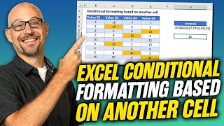
Jon, thank you for your video. It helped me figure out how to apply color to rows using a conditional format based on formulas comparing a constanvt value to a relative value in A. I created three rules, as you show it in your video I started each new rule on cell A2. Then I entered a formula to each rule as shown below: rule 1 formula ="Contract 101"=$A1 Format: light gray; Applies to =$A:$G rule 2 formula ="Contract 102"=$A1 Format: light blue; Applies to =$A:$G rule 3 formula = "Contract 103"=$A1 Format: light green; Applies to =$A:$G For years I had been using visual basic as a workaround but today I decided to google search a solution and I found your awesome video. Thank you for sharing it!. Great video!
I just was working on a budgeting sheet, so I can figure out if I really know what I'm spending my money on! This really helped with seeing if the numbers were higher or lower than they were previously, at a glance!
Hi I really Excited to learn excel with easy tips. I just start learning excel so I hope in future I will be provide all guidance learning excel.Thank you
Jon, This is a great tutorial. I struggled with this for a long time. You have a great way of explaining the procedure. But I still can't figure out how not to highlight blank cells. Can anyone help me with this?
When you are making the formula and selecting the cell in the data set, what do you do if the value that you want to highlight is not in the first cell of the data set? Does it have to be the first cell in the data set?
Hi Jon, here you're comparing cells in one row with a fixed reference. How do I compare cell in col A with cells in col D and copy and past the formula to apply the same conditional formatting to Col B to be compared with E and so on...I hope it's clear. Thanks in advance Giovanni
Excellent video. I had a follow-up question regarding this. Is it possible to have an additional version of this rule running in tandem, where one rule is authoritative over the other? For Example, Say we used the original formula from your tutorial, (if a value resides in E6 mark it as green throughout the worksheet) But then we add a separate, additional rule that does the exact same thing. For instance, if something resides in G6, mark it blue. We have E6 marking a value as green We have G6 marking a value as blue. How would we format it, so the rules don't conflict with each other if the same value exists in both E6 and G6? Is there a way to implement an "if/then" statement for G6, that states if the same value already exists and is marked in E6, ignore it?
HI i need help big time. I have done a baby guess chart. ie name , weight, time and so on. at the bottom i want to add all the bits in when he/she is born . i want it to highlight just the correct ones in that colomn. can you help i only have a couple of weeks left.
Jon, This video is really helpful.. Was wondering if we could format a row based on the value in the previous row..? imagine a row cell A10 and the previous row cell A9. I want to highlight the cell A10 if it is more than 1.2*A9 value.. I want to extend this to all the rows in a pivot table.. so this applies to A11 and A10 combination, A12 and A11 cells combination, and so on.. .. i.e. A11 gets highlighted if it is more than 1.2*A10.. and so on..
What I wanted to do is if cell M1 for example has any text or number then it would be highlighted a particular color of my choosing. I wanted the conditional format formula to also be in cell M1 and not be dependent on anything in another cell. So, using "Use a formula to determine which cells to format," I typed in "=counta(M1)>0. It didn't work. Then I noticed that Excel overrode my formula and stuck in some quotation marks into the formula, so it appeared as ="=counta(M1)>0". Without disturbing the formula I deleted the quotation marks, then clicked OK and Apply. Presto - it works.
Man, for some reason this is not working for me when the cell contains a day of the week (ie Monday, Tuesday, etc). Even when I'm using the preset "Highlight Cells > Text that Contains..." is not detecting any of the days.
Hi , and thanks for your help , and I have a question about speeding up and that is that , I want to just speed up my work book , but there things that are connected to this workbook , I saved them in just one workbook in another sheets , I wonder which possible way of saving and reloading data is faster ?! sheets or another workbook ?! and an another question is that i made a macro it was working well (i mean fast ) but after assigning it to button it didnt work well and it takes a period of time to complete the task why is that ?! i would really appreciate if u help me with these ! :) and consider more question are coming !!! ;)
I’m using this one long time before but maybe because too much data it’s not working for new rows I have to copy/paste the style to apply it again.. tomorrow will try to correct it’s . I’m using texts to match....
Hi Adel, I forgot to mention it in the video, but I'd recommend using an Excel Table (Ctrl+T) for the data range. The formatting rules should extend to new rows with a Table. However, it doesn't work with dynamic named ranges. This is something you can vote on to be fixed on the Excel Uservoice site. Here is the link. excel.uservoice.com/forums/304921-excel-for-windows-desktop-application/suggestions/10561194-conditional-formatting-apply-to-named-ranges I hope that helps. Thanks again and have a nice day! 🙂
Good evening. I believe that the word you would be looking for will take the place of the text he used. In this instance 6. Instead of 6, you type the word you are looking for. Try that. Hopefully, you figured it out already.
Not what I was looking for but still a good video. Wish there was a way to format cell with formula that is pulling data that is not entered yet (i.e. "#DIV/0!" = red font) to determine if there is missing data.
Hello everyone, I need help trying to share my master worksheet info with another workbook shared by 5 other people. I want to send each one a worksheet based on their name and whether or not it's highlighted on my master sheet. (MUST have their NAME in the cell and MUST be HIGHLIGHTED) I would love it if it was automatically updated whenever I add new info. Any help would be greatly appreciated.
Hi, please I need to know if there is an ability to use conditional formatting as if it is true gives a color and if false gives another color? Thanks for your support
I can't seem to get the formatting to work for time values. I'm trying to compare if the total hours (calculated in the cell) are greater than the hours put into another cell. It's for calculating billable hours on a job, and it adds up the billable hours. I want it to highlight the cells, if they are greater than the allowed number of billable hours, put in on a cell outside the table. I've tried putting it as =G3>N1, =$G$3>$N$1, =TIMEVALUE($G$3)>TIMEVALUE($N$1), etc. Any suggestions? I can't seem to find an answer to it anywhere. Thanks!
If you delete the reference cell for the formula, it doesn't know where to search. Edit the rule and put the new reference location in and the formula will work again.
Great question, Akala! 😊 Count the number of minimum values. If that amount is multiple, it would be 2 or more. Choose to highlight if the count of the minimum value is less than 2. If there are multiples, there will be no highlights. If the cell contains the minimum AND the minimum count is less than 2, then highlight. For example, for data in Cells A2:A7, the following formula would work in Conditional Formatting. =AND($A2=MIN($A$2:$A$7),COUNTIF($A$2:$A$7,MIN($A$2:$A$7))<2) Thanks again for the great question! 🙂
Great question, Santosh! This can be done with a macro. I do have a post on the AutoFilter method in VBA, but it does not address this question specifically. I'll add this to our list for future videos. Thanks! 🙂👍
i have a conditional format with a drop down list to highlight certain rows, how do i add in the if function to not highlight empty cells in my chart? this is my current rule =$G3=$L$2
Is it doing that when L2 is blank? It's doing that because it's highlighting whatever in G matches L2. Until someone suggests a solution, maybe use something in blank cells like X
Hello, do you have a tutorial on applying formatting to the rows of data that bolds the text and changes the text color if the "column" is more than a "%" of a "column"?
Didn't work for me! :-( Excel is sometimes very unpredictable does what it wants to do so may be its just the tool. Wish i could attach a screenshot here and show how random it is working
Hi Jon, I want to compare dates in column B with dates in column A and highlight the dates that are less than (earlier) column A dates in respective rows. Can this be done? Thanks.


I have watched dozens of videos and could not get it to work doing horizontal rows until I watched your video, THANK YOU!
Glad to hear that, Kelly! 😀
Worked great! Found this after hours and hours of searching... Thank you!
Glad it helped, Zilch! 😀
I was looking for exactly this. I was having trouble until I realized you said that the Check number you are searching for has to be in the same column as the trigger.
Thank you very much for posting this.
With the help of your video i finally managed to format rows containing a specific name,also adding aditional rules for more names and colors!
Thank you Jon.
love this video. i can never remember how to do this, but i now have a link to this saved so i can come back and watch it again every time i need to
Awesome! Thanks for bookmarking it and I'm happy to hear it helped. 🙂
Thank you Thank you Thank you! Just what I needed -- you made it so easy to follow!!!
Just watched this video as came up 'for you', and very informative. Thanks Paul
Glad you liked it!😀
Conditional formatting explain very simple way which has great practical use
Thanks Amit! 🙂
Everything was so well explained with all the relevant details made simple
. Thank you so much.
You're welcome, Mary! 😀
Awesome video. I used this in Google sheets and worked like a charm.
Jon, thank you for your video. It helped me figure out how to apply color to rows using a conditional format based on formulas comparing a constanvt value to a relative value in A. I created three rules, as you show it in your video I started each new rule on cell A2. Then I entered a formula to each rule as shown below:
rule 1 formula ="Contract 101"=$A1 Format: light gray; Applies to =$A:$G
rule 2 formula ="Contract 102"=$A1 Format: light blue; Applies to =$A:$G
rule 3 formula = "Contract 103"=$A1 Format: light green; Applies to =$A:$G
For years I had been using visual basic as a workaround but today I decided to google search a solution and I found your awesome video. Thank you for sharing it!.
Great video!
Thank you so much! This is maybe fifth first tutorial which i understood well and which works easily.
Great to hear that! 😀
This tutorial helped me. Thanks for posting
Thanks a million! Only your solution worked where about 10 I checked before all failed.
Very helpful! Saved me hours, thank you!
I really like your Tutorials! Great!
THANKS. IT IS REALLY GOOD TO LEARN.
I use this particular scenario a lot at work. Thanks!
Awesome! Thanks! 🙂
I just was working on a budgeting sheet, so I can figure out if I really know what I'm spending my money on! This really helped with seeing if the numbers were higher or lower than they were previously, at a glance!
Hi I really Excited to learn excel with easy tips. I just start learning excel so I hope in future I will be provide all guidance learning excel.Thank you
Thanks a lot. The video made my life easy. Great job
I got this, and was able to apply Really quickly!!! Thank you
thank you so much sir, great explanation and step by step. i really apricate you for this. kind regards;
Thanks for the feedback! 😀
Genius. Thanks man. This helped me a lot
Glad it helped! 😀
Fantastic explanation and examples!
Thanks Jon!
Very helpful. Thank-you.
Well explained thank you very much 🙏🏻
Thank you Jon. This is very much useful. Saved my day.
Glad it helped! 😀
It worked! Thank you so much! Lifesaver!
Glad it helped, @splattrick2432 ! 😀
very very interesting . Thank you jon
Great information! Keep up the good work, Jon!
Thanks for this great tutorial!!
Worked Great!!!
Thank you, it was very helpful
Glad to hear that! 😀
Many thanks Jon!
Thanks Zahid! 🙂
Thank You, good Sir.
Great video, very useful!
aaaaahhhh sir, lovely, made my whole life a lot more easier damnnn
Glad to hear that @superbrainy-fi1hv 😀
Awesome. Thank you!
Thank you for this, I was struggling trying to figure out why my formatting wasn't working
Thanks for this
i love you man
Thank you very much!! Very helpful for work! Great!!
Thanks Jon!
Thanks Yulin! 🙂
Thanks Sir
Very useful... Thank you so much
You are welcome! 😀
Thank you so much
Woow...thank you sir
Thanks Bro
Very nice. This will work great for my budget spreadsheet when determining a gain or loss on projected balance. Thank you!
Jon, This is a great tutorial. I struggled with this for a long time. You have a great way of explaining the procedure. But I still can't figure out how not to highlight blank cells. Can anyone help me with this?
When you are making the formula and selecting the cell in the data set, what do you do if the value that you want to highlight is not in the first cell of the data set? Does it have to be the first cell in the data set?
Hi Jon.. great lesson.. as always. Thanks for the many tips, tricks and insights that move us all forward a day at a time. Thumbs up!
Thanks so much, Wayne! 🙌
AMAZING vid, thanks for this tutorial.
Thanks Simoiya!
tysm u helped me so much 😭
Happy to help, Melba! 😀
This is great!
Thank you! 🙂
Hi Jon,
here you're comparing cells in one row with a fixed reference. How do I compare cell in col A with cells in col D and copy and past the formula to apply the same conditional formatting to Col B to be compared with E and so on...I hope it's clear.
Thanks in advance
Giovanni
Thank you
You're welcome! 😀
بالفعل انت شخص اكثر من رائع
I needed a help to highlight the all the impacted cells when we change the Main Cell. There are many cells gets effected if we do change in 1 Cell
Wow that's helpful
good one !!!👍👍👍👍👍
*It is very important and useful* - *ONTIME EDU*
Thanks Jon! You're doing amazing job. Can you do a video on data interpolation using excel. Thanks in advance!
Thanks, Uday! I appreciate your support! I'll add that to our list for future videos. 👍
Excellent video. I had a follow-up question regarding this. Is it possible to have an additional version of this rule running in tandem, where one rule is authoritative over the other?
For Example,
Say we used the original formula from your tutorial, (if a value resides in E6 mark it as green throughout the worksheet)
But then we add a separate, additional rule that does the exact same thing. For instance, if something resides in G6, mark it blue.
We have E6 marking a value as green
We have G6 marking a value as blue.
How would we format it, so the rules don't conflict with each other if the same value exists in both E6 and G6? Is there a way to implement an "if/then" statement for G6, that states if the same value already exists and is marked in E6, ignore it?
Thanks. Can you share about if function in the formatting condition?
where do I find the elevate excel series?
HI i need help big time. I have done a baby guess chart. ie name , weight, time and so on. at the bottom i want to add all the bits in when he/she is born . i want it to highlight just the correct ones in that colomn. can you help i only have a couple of weeks left.
Jon, This video is really helpful.. Was wondering if we could format a row based on the value in the previous row..? imagine a row cell A10 and the previous row cell A9. I want to highlight the cell A10 if it is more than 1.2*A9 value.. I want to extend this to all the rows in a pivot table.. so this applies to A11 and A10 combination, A12 and A11 cells combination, and so on.. .. i.e. A11 gets highlighted if it is more than 1.2*A10.. and so on..
i want to use conditional formatting if any value changes in that cell not relative to other cell
i don't get it... why does it apply formatting to whole row if we only compare to a single cell in the row?
What I wanted to do is if cell M1 for example has any text or number then it would be highlighted a particular color of my choosing. I wanted the conditional format formula to also be in cell M1 and not be dependent on anything in another cell. So, using "Use a formula to determine which cells to format," I typed in "=counta(M1)>0. It didn't work. Then I noticed that Excel overrode my formula and stuck in some quotation marks into the formula, so it appeared as ="=counta(M1)>0". Without disturbing the formula I deleted the quotation marks, then clicked OK and Apply. Presto - it works.
Man, for some reason this is not working for me when the cell contains a day of the week (ie Monday, Tuesday, etc). Even when I'm using the preset "Highlight Cells > Text that Contains..." is not detecting any of the days.
Hi , and thanks for your help , and I have a question about speeding up and that is that , I want to just speed up my work book , but there things that are connected to this workbook , I saved them in just one workbook in another sheets , I wonder which possible way of saving and reloading data is faster ?! sheets or another workbook ?! and an another question is that i made a macro it was working well (i mean fast ) but after assigning it to button it didnt work well and it takes a period of time to complete the task why is that ?! i would really appreciate if u help me with these ! :) and consider more question are coming !!! ;)
I’m using this one long time before but maybe because too much data it’s not working for new rows I have to copy/paste the style to apply it again.. tomorrow will try to correct it’s . I’m using texts to match....
Hi Adel,
I forgot to mention it in the video, but I'd recommend using an Excel Table (Ctrl+T) for the data range. The formatting rules should extend to new rows with a Table.
However, it doesn't work with dynamic named ranges. This is something you can vote on to be fixed on the Excel Uservoice site. Here is the link.
excel.uservoice.com/forums/304921-excel-for-windows-desktop-application/suggestions/10561194-conditional-formatting-apply-to-named-ranges
I hope that helps. Thanks again and have a nice day! 🙂
Hi Jon, is it possible to do this in VBA?
Awesome! I would love to know if or how this works when you're not looking for cells that have an exact value but rather contain a specific word.
Good evening. I believe that the word you would be looking for will take the place of the text he used. In this instance 6. Instead of 6, you type the word you are looking for. Try that. Hopefully, you figured it out already.
Instead of value,insert the word you want in " ". I did the same as you and i created 5 additional rules for 5 different words!
Not what I was looking for but still a good video. Wish there was a way to format cell with formula that is pulling data that is not entered yet (i.e. "#DIV/0!" = red font) to determine if there is missing data.
did you ever find this
Hello everyone, I need help trying to share my master worksheet info with another workbook shared by 5 other people. I want to send each one a worksheet based on their name and whether or not it's highlighted on my master sheet. (MUST have their NAME in the cell and MUST be HIGHLIGHTED) I would love it if it was automatically updated whenever I add new info. Any help would be greatly appreciated.
Hi, please I need to know if there is an ability to use conditional formatting as if it is true gives a color and if false gives another color?
Thanks for your support
did you ever find this
I can't seem to get the formatting to work for time values. I'm trying to compare if the total hours (calculated in the cell) are greater than the hours put into another cell. It's for calculating billable hours on a job, and it adds up the billable hours.
I want it to highlight the cells, if they are greater than the allowed number of billable hours, put in on a cell outside the table. I've tried putting it as =G3>N1, =$G$3>$N$1, =TIMEVALUE($G$3)>TIMEVALUE($N$1), etc.
Any suggestions? I can't seem to find an answer to it anywhere.
Thanks!
Nevermind! I figured it out. I did =$N$1
Hi, and what if I wanted to delete the orange box with the 2 in it now? I tried deleting mine and it messed up the entire formula
If you delete the reference cell for the formula, it doesn't know where to search. Edit the rule and put the new reference location in and the formula will work again.
hi, is there a way that you can highlight numbers that has decimal, and highlight numbers that are even and odds in the same data sheet?
you can use the greater then or less than formula please check my video on condition formating
HOW TO FEED THE VALUE SHOWING IN "SELECT MONTH"
What if you need the lowest value but highlight only if it is the single lowest, no multiples?
Great question, Akala! 😊 Count the number of minimum values. If that amount is multiple, it would be 2 or more. Choose to highlight if the count of the minimum value is less than 2. If there are multiples, there will be no highlights. If the cell contains the minimum AND the minimum count is less than 2, then highlight. For example, for data in Cells A2:A7, the following formula would work in Conditional Formatting.
=AND($A2=MIN($A$2:$A$7),COUNTIF($A$2:$A$7,MIN($A$2:$A$7))<2)
Thanks again for the great question! 🙂
The "<" would be a "less than" symbol. 😊
how to apply filter based on a cell value
Great question, Santosh! This can be done with a macro. I do have a post on the AutoFilter method in VBA, but it does not address this question specifically. I'll add this to our list for future videos. Thanks! 🙂👍
i have a conditional format with a drop down list to highlight certain rows, how do i add in the if function to not highlight empty cells in my chart? this is my current rule =$G3=$L$2
Is it doing that when L2 is blank? It's doing that because it's highlighting whatever in G matches L2. Until someone suggests a solution, maybe use something in blank cells like X
you can use the blank cell option
Hello, do you have a tutorial on applying formatting to the rows of data that bolds the text and changes the text color if the "column" is more than a "%" of a "column"?
Didn't work for me! :-( Excel is sometimes very unpredictable does what it wants to do so may be its just the tool. Wish i could attach a screenshot here and show how random it is working
What if the cells contain numbers with letters?? Example... A1, A2, A3... etc... how do you format that???
no problem you can use the text contains option check my video of conditional formatting
Conditional formatting explodes the size of the file
Ryan Reynolds?
Hi Jon, I want to compare dates in column B with dates in column A and highlight the dates that are less than (earlier) column A dates in respective rows. Can this be done? Thanks.
Thanks for the wonderful information..
Thank you
You're welcome 😀