Graphical Models 1 - Christopher Bishop - MLSS 2013 Tübingen

Вставка
- Опубліковано 27 гру 2013
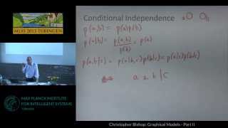
- This is Christopher Bishop's first talk on Graphical Models, given at the Machine Learning Summer School 2013, held at the Max Planck Institute for Intelligent Systems, in Tübingen, Germany, from 26 August to 6 September 2013.
Slides for this talk, in pdf format, as well as an overview and links to other talks held during the Summer School, can be found at mlss.tuebingen.mpg.de.


As a physicist, I really like his approach to machine learning. Very impressive slides and Feynman diagram was a good analogue . Thanks for MPI for IS sharing the series of video, I was a PhD student in MPI for physics.
wow. one of the best lecture on graphical model introduction. thank you
great lecture, many thanks for making this publicly available
I love how Mr. Bishop is always using “Pretty Woman” in the movie recommendation example. He must really love that move. :-)
Great content - thanks for sharing!
This is a kind of content that will be still relevant when deep learning will be superseded by the next big thing.
Awesome lecture! :)
Thanks for the great lecture! I like your book.
probability begin from 36:00
Thank you
lol thx
jiejie
Bold prediction about the future of Machine Learning especially given that Deep Learning has already become a thing at the time of this lecture.
How does the left graph on 1:14:48 represent PCA/ICA/linear regression?
It is simple. The node at the top is the latent variable (reduced dimension in PCA terms) and the node at the bottom is the observed variable (the original data size). In Regression, the node at the top is weight you're looking for, and the one at the bottom is data you observe. That said, this is very rough, lacks many PGM details like plates and shaded nodes and many other details.
Recommendable, but a very gentle introduction
Thanks for the wonderful video...One quick question ..why did we start with joint probability in graphs? I mean in lecture we saw product rule, sum rule, conditional probability etc...but then in graphs we started factorization using joint probability. Why? What is the idea behind doing/finding joint probability of x1..xp? I have already checked over net that joint prob would give an idea about which variable are dependent on other..but then how is this related to our graph learning?..Many thanks in advance
Nice!💯
Is the product rule backwards in the butler Cook example?
world-class
Great lecture...just want mention that @1:01:59, for "the graphs in the essence are adding nothing to the equations...", I guess Judea Pearl may have a different opinion, from causality's point of view, that graphs do add something explicitly to the algebraic equations.